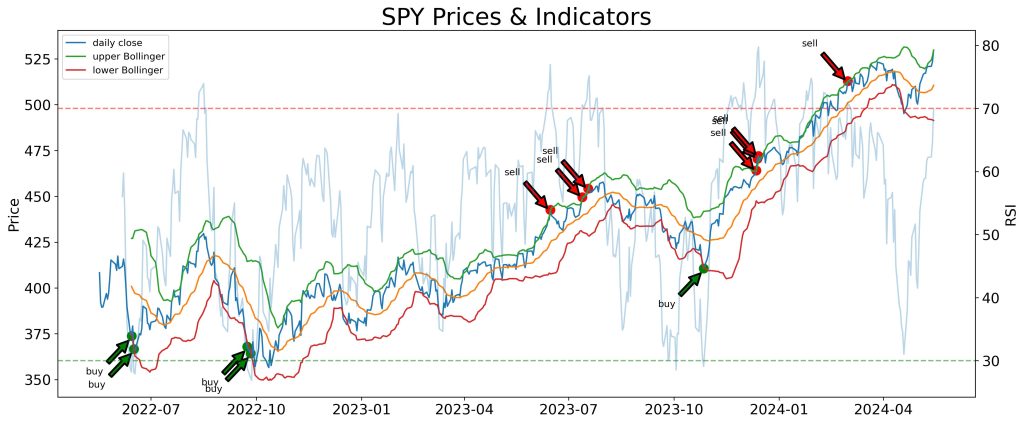
I use Python with library packages including Pandas, NumPy, and matplotlib, as well as Yahoo Finance, and ta to show buy and sell points of some popular stocks. I will be looking at SPY (ETF), NVDA, AMD, MSFT, META, in particular. Coding is done on a Jupyter Notebook, as shown below. I will also briefly explain the code.
The following figure shows a 2-year price history of SPY from Yahoo Finance, which includes HLOC as well as volume and adjusted close (taking into dividends and stock split). Of the stocks listed above, only AMD has no difference between ‘Adj Close’ and the actual closing price. Some of them have pretty significant difference. I choose to use the closing price to avoid confusion.
For the Bollinger band, I use a 20-day moving average (ma) and 2 standard deviation (std). I think 20 day ma makes sense because that’s 1-month of trading. 2-std of a normal distribution will cover 95% of the data points. In other words, only 5% of the time, stocks will trade out of the Bollinger band, assuming stock prices are normally distributed around the mean (ma).
For the RSI, I use the common 14-day average.
Below is the 2-year chart of SPY’s daily close. Arrows point at the buy and sell points. Here I define a sell point when the price is above the upper band and the RSI is over 70 (the red horizontal line). On the other hand, when the price falls below the lower band and the RSI is below 30, it’s a buy point.
It appears that stock prices are well confined between the upper and lower bands. The problem is that the Bollinger bands are moving averages of the past pricing.

